Different ways to read csv file in python

Introduction

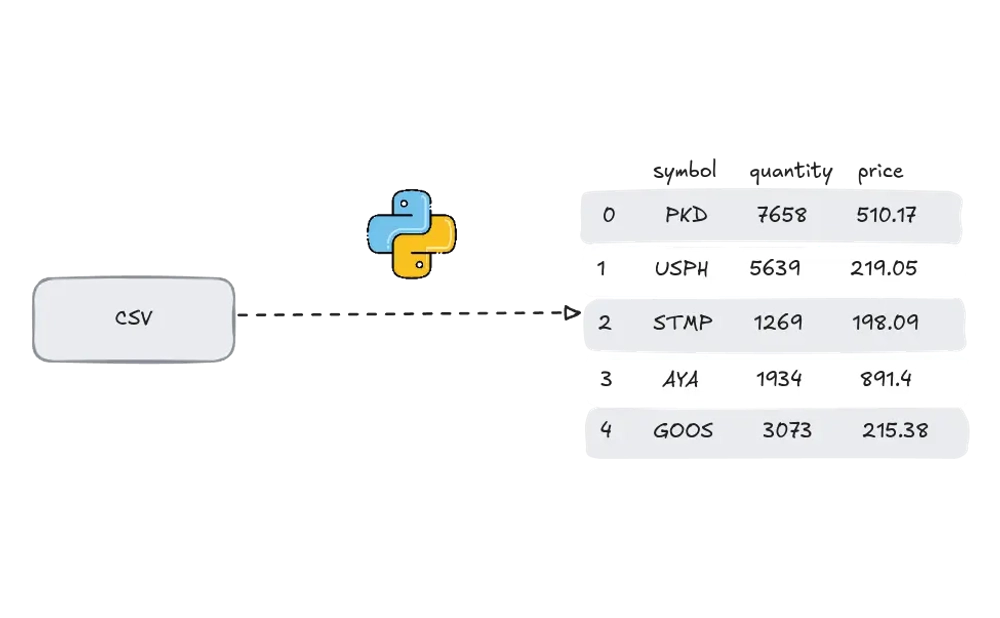
There are several ways to read CSV (Comma-Separated Values) files in Python, each with advantages and use cases.

In this post, I have compared csv, pandas, numpy, open function with split, pyexcel, dask and tablib libraries.

• open Function with split: Basic and straightforward for simple CSV files.
• csv: Part of the standard library, suitable for simple CSV processing.
• pandas: Powerful and flexible, ideal for data analysis and manipulation.
• numpy: Useful for numerical computations and simple CSV files.
• pyexcel: High-level interface for various spreadsheet formats.
• tablib: Simple and consistent interface for tabular data.
• dask: Designed for parallel computing and handling large CSV files.

Here is a detailed explanation of these methods with examples:

1. Using the open Function with split

For simple CSV files, you can use the built-in open function along with string manipulation methods like split.

Consider a file named MOCK_DATA.csv that contains comma-delimited csv data as shown below:

trade_id,stock_symbol,quantity,purchase_price,sale_price,purchase_date,sale_date,profit,profit_percentage,trade_type
1,PKD,7658,510.17,323.29,8/30/2012,12/14/2013,-186.88,-36.6309269459199874551620048,buy
2,USPH,5639,219.05,229.82,12/22/2013,2/21/2011,10.77,4.9166856881990413147683177,buy
3,STMP,1269,198.09,436.76,7/18/2015,1/31/2013,238.67,120.4856378413852289363420667,buy
4,AYA,1934,891.4,909.88,3/9/2009,10/9/2018,18.48,2.0731433699798070450975993,buy
5,OPHC,7746,428.47,860.57,4/8/2013,3/3/2003,432.1,100.8472005041193082362825869,buy
6,SSD,6154,764.9,499.37,11/19/2018,8/9/2008,-265.53,-34.7143417440188259903255327,sell
7,ALL^D,6427,677.69,528.55,8/21/2019,10/7/2017,-149.14,-22.0071123965234841889359442,buy
8,NGHCO,8462,592.29,945.79,5/12/2001,9/6/2015,353.5,59.6836009387293386685576322,buy
9,GOOS,3073,215.38,396.14,2/8/2010,8/3/2002,180.76,83.9260841303742223047636735,buy
10,SCHW,5571,77.23,706.23,12/28/2013,9/4/2001,629.0,814.4503431309076783633303121,buy

# Read CSV file using open and split
with open("MOCK_DATA.csv", "r") as file:
    lines = file.readlines()
    for line in lines:
        row = line.strip().split(",")
        print(row)

2. Using the csv Module

The csv module is part of Python’s standard library and provides functionality for reading and writing CSV files.

import csv

# Read CSV file using csv.reader
with open("MOCK_DATA.csv", "r") as file:
    reader = csv.reader(file)
    for row in reader:
        print(row)

# Read CSV file using csv.DictReader
with open("MOCK_DATA.csv", "r") as file:
    reader = csv.DictReader(file)
    for row in reader:
        print(row)

3. Using the pandas Library

Pandas provide various functions for manipulating and transforming data, making it easy to clean, filter, and aggregate CSV data. pandas integrate well with other Python libraries, such as numpy for numerical computations and matplotlib for data visualization. pandas can read CSV data from different sources, including files, URLs, and strings. It supports multiple options for handling different CSV formats and structures.

Example 1: Read the CSV File into DataFrame

import pandas as pd

# Read CSV data with custom options
df = pd.read_csv(
    "MOCK_DATA.csv", delimiter=",", header=0, parse_dates=["purchase_date", "sale_date"]
) 
print(df)

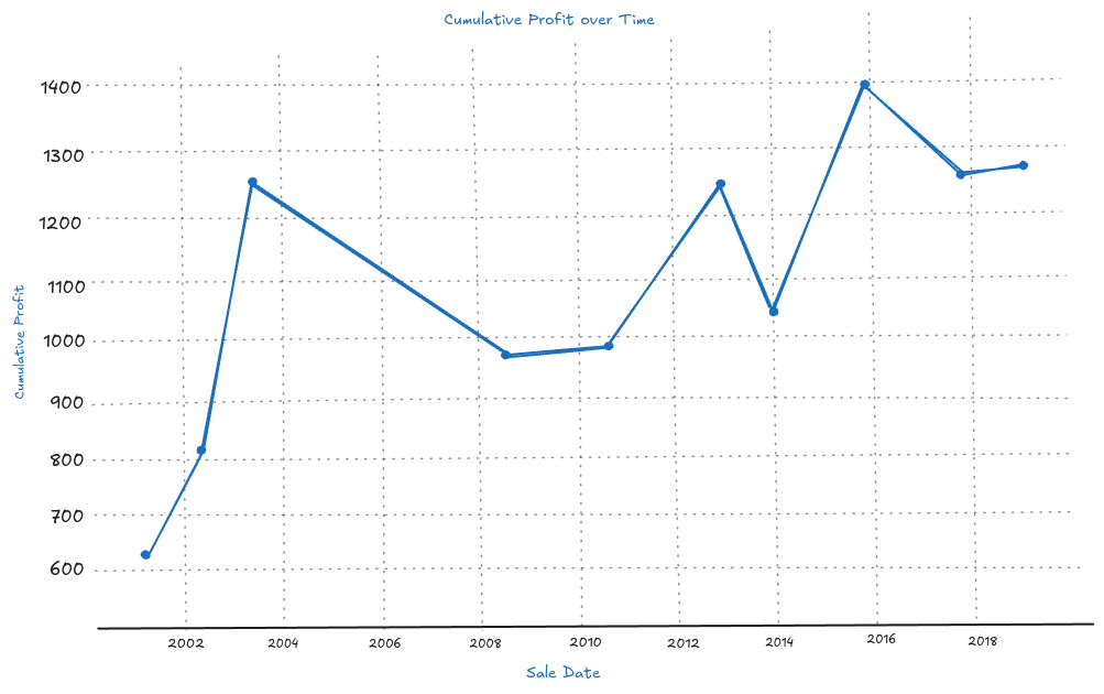
Example 2: Plot charts using matplotlib library

You must install matplotlib and pyqt6(if running in the terminal) libraries to plot charts.

pip install matplotlib, pyqt6

a. Plotting cumulative profit over time

import matplotlib.pyplot as plt

# Ensure the 'purchase_date' and 'sale_date' columns are in datetime format
df["purchase_date"] = pd.to_datetime(df["purchase_date"])
df["sale_date"] = pd.to_datetime(df["sale_date"])

# Sort the DataFrame by sale date
df = df.sort_values(by="sale_date")

# Calculate cumulative profit
df["cumulative_profit"] = df["profit"].cumsum()

# Plot cumulative profit over time
plt.figure(figsize=(10, 6))
plt.plot(df["sale_date"], df["cumulative_profit"], marker="o", linestyle="-")
plt.xlabel("Sale Date") 
plt.ylabel("Cumulative Profit")
plt.title("Cumulative Profit Over Time") 
plt.grid(True)
plt.xticks(rotation=45)
plt.show()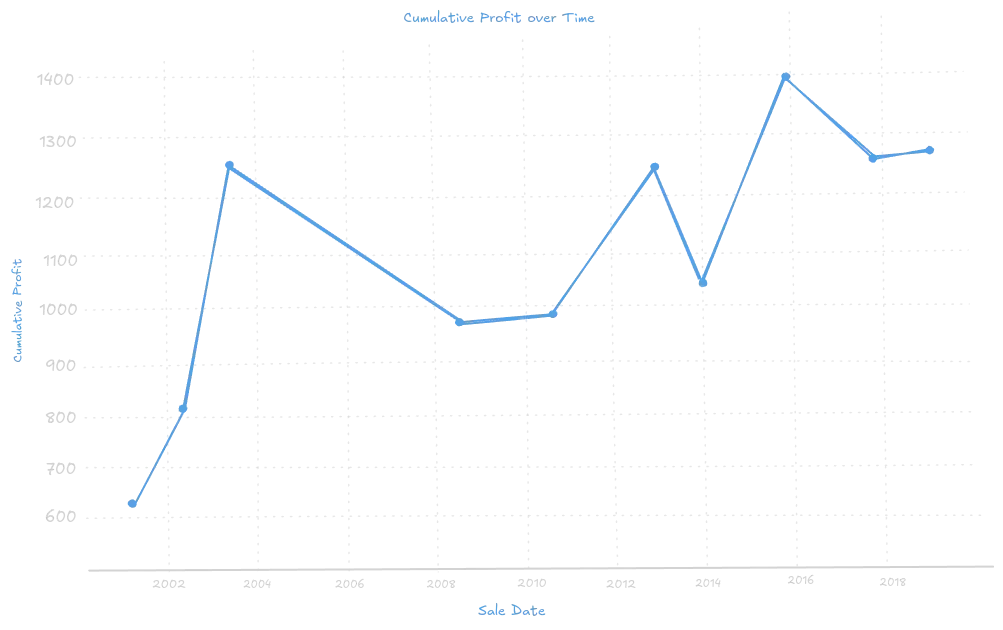

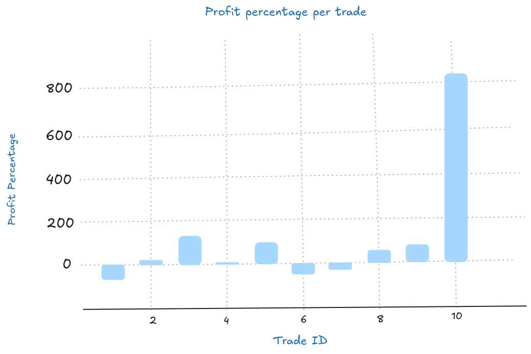
b. Plotting profit percentage

# Plot profit percentage
plt.figure(figsize=(10, 6)) 
plt.bar(df["trade_id"], df["profit_percentage"], color="skyblue")
plt.xlabel("Trade ID")
plt.ylabel("Profit Percentage")
plt.title("Profit Percentage per Trade")
plt.grid(True)
plt.show()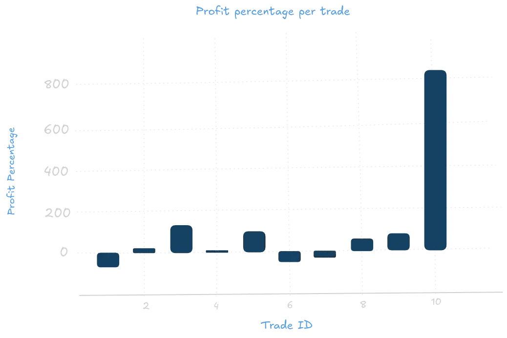

4. Using the numpy Library

NumPy is a powerful library for numerical data processing in Python. While it is not specifically designed for CSV data processing, it can be used in conjunction with other libraries like pandas to handle and manipulate numerical data from CSV files efficiently. NumPy provides efficient data structures like ndarray (n-dimensional array) data structure, which is highly efficient for numerical computations and data manipulation. It also offers a wide range of mathematical functions, making it a valuable data analysis and manipulation tool. NumPy provides various options for customizing the reading of CSV files, such as specifying delimiters, handling headers, and parsing dates.

NumPy provides the genfromtxt and loadtxt functions for reading CSV data into arrays.

import numpy as np

# Read CSV data using genfromtxt
data = np.genfromtxt('trading_data.csv', delimiter=',', skip_header=1)
print(data)

Reading CSV Data with pandas and Converting to numpy Array

import pandas as pd
import numpy as np

# Read CSV data using pandas
df = pd.read_csv('trading_data.csv')

# Convert DataFrame to NumPy array
data = df.to_numpy()
print(data)

Aggregating Data (Calculate the total profit)

import numpy as np
import pandas as pd

# Read CSV data using pandas
df = pd.read_csv("MOCK_DATA.csv")

# Convert DataFrame to NumPy array
data = df.to_numpy()

# Calculate the total profit
total_profit = np.sum(data[:, 7].astype(float))
print(total_profit)

5. Using the pyexcel Library

pyexcel is a Python library for reading, writing, and manipulating data in various spreadsheet formats, including CSV, Excel (XLS and XLSX), and ODS (OpenDocument Spreadsheet). Pyexcel can be integrated with other data processing libraries like Pandas to leverage its strengths. For example, you can read CSV data using pyexcel and then convert it to a pandas DataFrame for further analysis.

import pyexcel as p

# Read CSV data from a file
records = p.get_records(file_name="MOCK_DATA.csv")

# Filter records where 'profit_percentage' is greater than 5
filtered_records = [record for record in records if record["profit_percentage"] > 5]
for record in filtered_records:
    print(record)

6. Using the tablib Library

tablib is a Python library that handles tabular data in various formats, including CSV, Excel (XLS and XLSX), JSON, and YAML. tablib is particularly useful when working with multiple data formats interchangeably. tablib allows you to manipulate and transform data, making it easy to clean, filter, and aggregate CSV data. Tablib can be integrated with other data processing libraries like Pandas to leverage its strengths.

import tablib

# Read CSV data from a file
dataset = tablib.Dataset().load(open("MOCK_DATA.csv").read())

# Filter rows where 'profit_percentage' is greater than 5
filtered_dataset = tablib.Dataset(headers=dataset.headers)
for row in dataset:
    if float(row[-2]) > 5:
        filtered_dataset.append(row)

# Display the filtered data
for row in filtered_dataset:
    print(row)

7. Using the dask Library

Dask is a powerful parallel computing library in Python that is designed to handle large datasets that may not fit into memory. It achieves this by breaking down computations into smaller tasks that can be executed in parallel across multiple cores or even distributed across a cluster of machines. Dask can be particularly useful for processing large CSV files, as it allows you to perform operations on the data without loading the entire dataset into memory. Dask provides a DataFrame API similar to pandas, making it easy to transition from pandas to Dask for large-scale data processing.

import dask.dataframe as dd

# Read CSV data into a Dask DataFrame
df = dd.read_csv("MOCK_DATA.csv")

# Display the first few rows of the DataFrame
print(df.head())

# Filter rows where 'profit_percentage' is greater than 5
filtered_df = df[df["profit_percentage"] > 5]

# Calculate the total profit
total_profit = filtered_df["profit"].sum().compute()
print(f"Total Profit: {total_profit}")

Difference between Dask and Apache Spark.

Dask and Apache Spark are both powerful distributed computing frameworks designed to handle large-scale data processing tasks. However, they have different design philosophies, strengths, and use cases. Here are the key differences between Dask and Spark:

	Dask	Apache Spark
Design Philosophy	Dask is designed to be a lightweight, flexible, and Python-native parallel computing library. It aims to provide a familiar Pythonic interface and integrate seamlessly with the Python ecosystem, including libraries like NumPy, Pandas, and scikit-learn. Dask can scale from a single machine to a cluster of machines.	Apache Spark is a unified analytics engine for large-scale data processing. It is designed to handle big data workloads and provides rich libraries for SQL, streaming, machine learning, and graph processing. Spark is built on the Java Virtual Machine (JVM) and supports multiple languages, including Python (via PySpark), Scala, Java, and R.
Ecosystem Integration	Dask integrates tightly with the Python ecosystem and can work with existing Python libraries and tools. It provides a familiar API similar to Pandas, making it easy for Python developers to transition to distributed computing.	Spark has a broader ecosystem and supports multiple languages and APIs. It provides a rich set of libraries, including Spark SQL, Spark Streaming, MLlib (for machine learning), and GraphX (for graph processing).
Performance	Dask can be highly performant for Python-native workloads and can leverage Python’s Just-In-Time (JIT) compilation capabilities. It is well-suited for tasks that involve complex Python objects and workflows.	Spark is optimized for large-scale data processing and can handle petabytes of data efficiently. It uses in-memory computing to achieve high performance and can leverage distributed storage systems like HDFS.
Fault Tolerance	Dask provides basic fault tolerance by retrying failed tasks. It relies on the underlying scheduler (e.g., Dask Distributed) for more advanced fault tolerance mechanisms.	Spark has built-in fault tolerance and can automatically recover from failures by re-executing lost tasks. It uses a lineage graph to track the dependencies between tasks and can recompute lost data.
Deployment	Dask can be deployed on a single machine, local, or cloud-based cluster. It can be integrated with existing HPC (High-Performance Computing) environments and can leverage job schedulers like SLURM or PBS.	Spark can be deployed on various cluster managers, including YARN, Mesos, Kubernetes, and Spark’s standalone cluster manager. It is commonly used in cloud environments like AWS EMR, Google Cloud Dataproc, and Azure HDInsight.
Use Cases	Dask is well-suited for data science and machine learning workflows that involve complex Python code and libraries. It is often used to parallelize existing Python code and tasks requiring tight integration with the Python ecosystem.	Spark is well-suited for large-scale data processing, real-time analytics, and machine learning at scale. It is commonly used in enterprise environments for ETL (Extract, Transform, Load) pipelines, data warehousing, and big data analytics.

Find out more about Apache Spark in this post.

Each method has its strengths and is suitable for different use cases. The choice of method depends on your specific requirements, such as the complexity of the CSV file, the need for data manipulation, and the data size. All the code mentioned in this blog post can be found in this Git repository.